Curriculum 'User Guide Viedoc 4'
Dynamic randomization Download PDF
1 Introduction
- The underlying theory for the dynamic randomization in Viedoc™ is described in the following articles:
- Pocock S.J. and Simon R. Sequential treatment assignment with balancing for prognostic factors in the controlled clinical trial. Biometrics 1975;31:103-115.
- Miller E. Probability sharing in a modified Pocock-Simon method.12th Int. Conf. of S.C.M.A Jun 22, 2005.
- The method involves determining the amount of imbalance for each of the prognostic factors,
hypothetically assigning the next subject to each treatment group, and then assigning that
subject to the treatment group which will minimize the treatment assignment imbalances.
The original statement of the minimization method was deterministic, in that random number values were only used in tie-breaking situations. In the modified Pocock-Simon method implemented in Viedoc every randomization decision is dependent on a random number. Donald E. Knuth's subtractive random number generator algorithm is used. (D. E. Knuth. "The Art of Computer Programming, volume 2: Seminumerical Algorithms". Addison-Wesley, Reading, MA, second edition, 1981).
2 Concepts and algorithms
- The same notations as in the above mentioned article are used.
- Factor weight - a factor relative importance can be adjusted by setting a weight on the factor (an integer value greater than zero). For example, if it is more important to achieve balance in the Gender factor than in the Age factor, then a weight of 2 could be set on Gender and a weight of 1 set on Age.
- Outcome weight - also referred to as the allocation ratio, this sets the desired division of treatments to be allocated. For example, say we have three treatments A, B and C. If we would like treatment A to be allocated 50% of the time, and treatments B and C 25% of the time respectively, we would set the outcome weights as follows: Treatment A: 2, Treatment B: 1, Treatment C: 1.
- D - is the amount of variation in the set of values for a factor, i.e. it shows the imbalance in the set. The table in the picture illustrated below in section 8. Behind the scenes calculations shows and explains how this is calculated.
The amount of variation can be calculated as:- Range - this is the difference between the highest and the lowest values in the set.
- Range Squared - the square of the range as calculated above.
- G - represents the total amount of inbalance and is calculated by multiplying the factor weight by the D and adding them up across all factors. This means that, if a factor has a higher weight, it is more important to have it in balance - so if there is an imbalance the factor weight will enhance the difference to make it more unfavourable. If calculating the amount of variation as range square, the range is squared before any factor weight is applied.
G is calculated as the sum of {dik}, where dik is the lack of balance among treatment assignments. The weighted sum is used when some prognostic factors are considered more important than others. The factor weights are to be specified in connection with the Viedoc setup. - P - The probability with which to select the treatment that minimizes the imbalance.
For the following formulae: N = number of treatments, p = probability. The probability (p) is a decimal between 0 and 1 which is defined by the statistician.
- If all the Gs are the same for all treatments, then the probability will be the same for each treatment, i.e. p/N.
- If one treatment has the lowest G, then it will have its probability as p. The remaining treatments will split the remaining probability, i.e. (1 - p)/(N - 1)
- If one or more treatments share the lowest G value, then we first calculate what the remaining non-favoured treatments will get and then split the remainder between the favoured treatments.
- Using the above algorithms, a frequency table is calculated for each new patient to be randomized. A random number greater than or equal to 0 and less than 1 is then generated using a seed value based on the number of ticks to represent the current date. Using the Ps and this random number a treatment index is chosen and the patient is thereby assigned this treatment.
- The main workflow in Viedoc is as follows (illustrated with a particular example in the following sections):
- Configure the dynamic randomization by entering the input factors, outcomes, factor weights, allocation ratio, probability and choose if D should be calculated as range or as range square.
- When a new subject is added and it should be assigned a treatment as a result of the randomization, the following calculations are performed:
- Hypothetically assign the subject to each of the possible outcomes (treatments) and calculate for each treatment, for each of the input factors:
- Add 1 to the current treatment count
- Divide all set counts by the corresponding treatment allocation ratio
- Calculate the variance (D) (that was defined as range or range square) for each of the prognostic factors
- Calculate the total amount of imbalance (G) for each of the possible outcomes (treatments)
- Calculate the probability (P) with which to select the treatment that minimizes the imbalance for each of the possible outcomes
- Generate a random number greater than or equal to 0 and less than 1.
- Assign the outcome (treatment) that minimize the imbalance according to the calculated probabilities and the random number.
3 Use case description
- Let's consider the following scenario:
We want to assign a treatment on a randomized basis, depending on two factors: subjects gender (male/female) and age (<=30 or >30). - We have three treatments: A, B and C, and we want treatment A to be allocated 50% of the time, and treatments B and C 25% of the time respectively.
- The sections below describe the steps to go through for setting up the dynamic randomization in Viedoc for this particular case and how it works.
4 Forms set up in Viedoc Designer
- We have two main forms that we are going to use in our example:
- Add subject form - with two items capturing the gender and age
- Treatment form - with three items: gender and age defined exacly of the same type as in the Add subject form, and with a function defined for each that gather the item value from the filled in Add subject form. The third item is a radio button with three choices for the treatment (A, B, C) that will get a value as a result of the randomization.
5 Set up randomization in Viedoc Designer
- The step by step instructions on how to set up randomization in Viedoc Designer can be found in section 8. Randomizations at Study Settings.
- In this case, we select:
• Event, Activity and Form for our defined Treatment form. • Factors - the gender and age items in the Treatment form. • Outcomes - the Treatment item that is going to be populated as a result of the randomization.
6 Configure dynamic randomization in Viedoc Admin
- The step by step instructions on how to set up randomization in Viedoc Admin can be found at Configuring randomizations
- We have the Factors and the Outcomes as previously defined in Viedoc Designer.
- We choose Dynamic as a Randomization method.
Note! The dynamic method can only be chosen if the following criteria are met: • Only one outcome is chosen • All the selected input factors, as well as the outcome must have a code list.
Note! Make sure that, in case of choosing Country or Study site as Scope, you do not use country or site respectively as input factor(s). - We configure the dynamic randomization as follows:
- Variation method - Range (the difference between the highest and the lowest values in the set.)
- Probability - 800 (the equivalent of 80%)
- Factor weights - in our example, it is more important to achieve balance in the Gender factor, so we set it to 2 for the Gender and 1 for the Age.
- Allocation ratio - as we want treatment A to be allocated 50% of the time, and treatments B and C 25% of the time respectively, we set this to 2 for treatment A, and to 1 for B and C.
- Max slots (per list)
7 Randomize in Viedoc Clinic
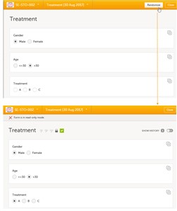
- In Viedoc Clinic, after filling in the subject information, when opening the Treatment form, the Gender and Age values are automatically populated from the Add subject form, and the Treatment item is to be filled in.
- After clicking the Randomize button in the upper right corner of the window, a value will be assigned for the Treatment item, according to the randomization settings previously performed.
Note! The form becomes read only after the randomization. This means that no item in the Treatment form will be editable, not even in case one of the Gender or Age values changes in the original form (Add subject form).
8 Behind the scenes calculations
- For our example above, considering the notations and explanations in section 2. Concepts and algorithms, we are going to explain how the calculations are made for assigning one of the three treatments (A, B or C) each time a new subject is added
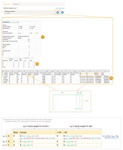
- After having added a few subjects and randomizing, we are going back to Viedoc Admin and open the randomization window. In the bottom we can see a Randomization list that can be opened by clicking on the eye icon. The xls file i downloaded and for our example, looks as in the picture. The xls file has three sheets:
- Configuration (1) - shows all the parameters we have previously configured for our randomization in Viedoc.
- Current distribution (2) - a summary of the number of entries classified by each of the input factors and the outcome respectively. In our example, we can see, for each of the treatments (A,B,C), how many subjects were assigned to it, of which how many are males/females and how many are aged <=30, respectively <30.
- Slots (3) - one row for each added subject, with the respective calculated values and the treatment assigned accordingly.
- Let's consider the first added subject and take a look into how the first set of calculations is performed in order to assign a randomized treatment.
- All the values in the distribution table (illustrated by (2) in the image) are equal to 0 at start point.
We are adding a first subject with Gender = Female and Age > 30. For this, we follow the workflow for calculating D, G and P for each of the three possible outcomes (treatments in our case).
We are going to use the following notations:
• wG - factor weight for gender = 2 • wA - factor weight for age = 1
• rA - allocation ratio for treatment A = 2 • rB - allocation ratio for treatment B = 1 • rC - allocation ratio for treatment C = 1
• dAM - variance for treatment = A and gender = male • dAF - variance for treatment = A and gender = female • dA(<=30) - variance for treatment = A and age <= 30 • dA(>30) - variance for treatment = A and age > 30 • dBM, dBF, dB(<=30), dB(>30), dCM, dCF, dC(<=30), dC(>30) - variances for treatment B, respective C, in the same manner as described above for treatment A. - We start by hypothetically assigning each of the three treatments and calculating the variances for each one. As the subject to be added is a female with age > 30, we only have to calculate the variances for those factor values.
Assuming that treatment A would be assigned, we add 1 in the distribution table for the treatment A, Female column and age > 30. The variances for each factor are calculated as below and illustrated by the last table in the image:- dAF = 1/ rA - 0 = 1/2 = 0.5 (one female subject was added, which makes the highest value in the distribuion table corresponding to the Female column = 1 and the lowest = 0)
- dA(>30) = 1/ rA - 0 = 1/2 = 0.5 (one subject was added with age > 30, which makes the highest value in the distribuion table corresponding to the >30 column = 1 and the lowest = 0)
- dBF = 1/ rB - 0 = 1 (one female subject was added, which makes the highest value in the distribuion table corresponding to the Female column = 1 and the lowest = 0)
- dB(>30) = 1/ rB - 0 = 1 (one subject was added with age > 30, which makes the highest value in the distribuion table corresponding to the >30 column = 1 and the lowest = 0)
- dCF = 1/ rC - 0 = 1 (one female subject was added, which makes the highest value in the distribuion table corresponding to the Female column = 1 and the lowest = 0)
- dC(>30) = 1/ rC - 0 = 1 (one subject was added with age > 30, which makes the highest value in the distribution table corresponding to the >30 column = 1 and the lowest = 0)
- Calculate the total amount of imbalance for each of the three possible treatments to be assigned:
- GA = dAFwG + dA(>30)wA = 0.5*2 + 0.5*1 = 1.5
- GB = dBFwG + dB(>30)wA = 1*2 + 1*1 = 3
- GC = dCFwG + dC(>30)wA = 1*2 + 1*1 = 3
- Calculate the probability (p) - we have set the probability to 0.8 in our example.
The treatment with the lowest G (in our case A) will get the highest p (in our case 0.8), and the remainder will be split between the other two. This means that:
- pA = 0.8 (meaning greater than or equal to 0 and less than 0.8)
- pB = 0.1 (meaning greater than or equal to 0.8 and less than 0.9)
- pC = 0.1 (meaning greater than or equal to 0.9 and less than 1)
- A random number between 0 and 1 is generated using Donald E. Knuth's subtractive random number generator algorithm.
In our example, the number is the one we can see in table (3) in the image under Random column, for the first entry = 0.93...
Considering the probabilities and the random number, the treatment C will be assigned to the first subject, as illustrated in the image.